Is 3x Nasdaq-100 exposure the best way to maximize long-run wealth? Multiplying the index’s total gain by three cannot answer that question. Daily compounding, recovery after losses and the financing cost of extra exposure determine what happens to the original investment.
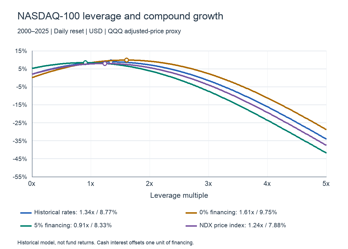
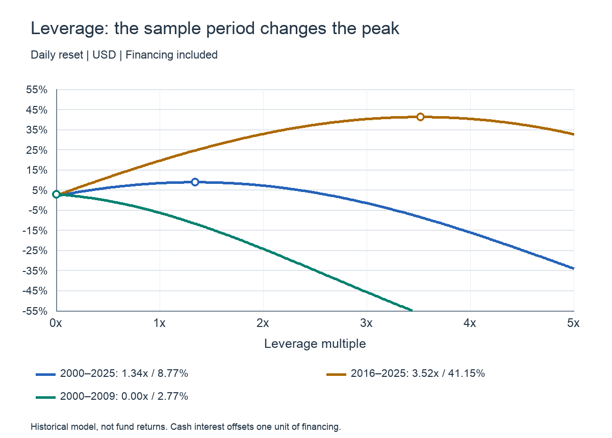
Our distribution-adjusted Nasdaq-100 ETF proxy produces a clear result: for 2000–2025, compound annual growth peaked at 1.34x leverage and 8.77% a year. For 2016–2025 alone, it peaked at 3.52x and 41.15%. Strong bull markets reward daily leverage. Including the dot-com collapse changes the full-period result dramatically.
A Japanese fund combines 3x equities with 1x USD/JPY
au Asset Management’s announcement schedules the launch of auAM Triple NASDAQ100 Unhedged for October 15, 2026. Its prospectus describes approximately three times daily USD equity exposure and one times USD/JPY exposure, using index futures and other instruments.

The critical distinction is three times the daily move, not three times the long-term return. After each day’s gain or loss, exposure is reset against the changed asset value. The sequence of daily gains and losses determines compounded growth.
Geometric growth captures the cost of large fluctuations
An index gaining 10% and then losing 9.09% almost returns to its starting point. Ignoring financing, a daily 3x strategy gains 30% and then loses 27.27%. An initial 100 becomes 130 and then approximately 94.55: a loss of 5.45% despite a flat underlying index.
Persistent gains work differently. The next positive return is earned on a larger balance, and leverage amplifies both the daily gain and the compounding. That benefit competes with the loss from repeated fluctuations, creating a peak in the growth curve. Our horizontal axis runs from 0x to 5x; the vertical axis is annualized geometric return, or CAGR, calculated from compounded daily factors over the actual calendar period. It is not the arithmetic average of daily returns multiplied by 365.
The full-period peak is 1.34x; the price index peaks at 1.24x
We used 6,539 daily returns from the first trading day of 2000 through the end of 2025. The primary series is distribution- and split-adjusted QQQ, a proxy for reinvested Nasdaq-100 equity returns. QQQ’s own expenses remain reflected in prices. We also calculated the same model directly from the Nasdaq-100 price index, NDX. Without dividends, its peak is 1.24x and 7.88% annual growth—again well below 3x leverage.
| Leverage | Annual compound return | Maximum drawdown |
|---|---|---|
| 1x | +8.30% | -82.96% |
| 2x | +7.08% | -98.69% |
| 3x | -1.62% | -99.97% |
The main model’s CAGR is 8.30% at 1x, 7.08% at 2x and −1.62% at 3x. The 3x strategy’s maximum drawdown is approximately 99.97%. Drawdown measures the decline from a wealth peak to a subsequent trough, not an annual return. After severe losses in the 2000s, later gains compound on a much smaller capital base.
For the NDX price series, the corresponding growth rates are 7.66%, 5.55% and −4.06%. Dividend treatment changes the levels, but not the finding that 3x failed to maximize growth over this full sample. This is a daily-reset leverage model using historical equity returns, not the performance history of the new Japanese fund.
Financing is separate from a fund’s management fee
Financing is embedded in index futures pricing. CME’s fair-value explanation identifies the cash index, interest rates, dividends and time to expiration as relevant inputs. Extra exposure has a carrying cost even when equities do not rise.
Subtracting three times the cash rate from a 3x portfolio would ignore interest earned on collateral. Assuming collateral and financing earn and pay the same rate, our model uses daily return = L × equity return − (L−1) × cash return. At 3x, the extra two units bear net financing; at 1x, there is no extra charge. Below 1x, uninvested cash earns interest.
We use FRED’s three-month US Treasury bill yield, TB3MS. Each trading interval uses the previous month’s yield, multiplied by elapsed calendar days divided by 365. Weekends and holidays still accrue interest. This is a symmetric financing/collateral approximation. Actual products also face financing spreads, their collateral investment terms, management fees and trading or roll costs. We apply the charge to unleveraged equity returns, not to TQQQ or futures prices that already include financing.
Hold the historical QQQ returns unchanged but fix financing at 0%: the peak becomes 1.61x and 9.75% annual growth. At a constant 5%, it falls to 0.91x and 8.33%. The 3x CAGR changes from +2.20% at 0% financing to −7.55% at 5%. Higher rates raise the hurdle for extra equity exposure and move the growth-maximizing multiple left. With cash earning 5%, a model portfolio below 1x can outperform full equity exposure.
The recent decade peaks at 3.52x: the sample matters
| Sample | Best multiple in 0–5x | Maximum CAGR | 3x CAGR |
|---|---|---|---|
| 2000–2009 | 0.00x (cash) | 2.77% | -45.79% |
| 2010–2019 | 5.00x (search boundary) | 64.03% | +47.84% |
| 2020–2025 | 2.87x | 34.85% | +34.77% |
| 2016–2025 | 3.52x | 41.15% | +40.13% |
For 2010–2019, growth is highest at the 5x boundary of our 0–5x search. That is a boundary result, not proof of an interior optimum at exactly 5x. The 2020–2025 peak is 2.87x; the 2016–2025 peak is 3.52x. For 2000–2009, 0x—cash earning the bill-rate proxy—wins.
These differences explain what leverage amplifies. Strong persistent returns, moderate daily volatility and cheap financing support higher multiples. Deep declines, large back-and-forth moves and expensive financing shift the peak lower. Place the recent decade beside the dot-com-inclusive sample to see the market conditions that make 3x successful.
A useful approximation is g(L) ≈ Lμ−(L−1)r−½L²σ², where μ is annual arithmetic equity return, r the cash rate and σ annual volatility. The approximate growth-optimal multiple is (μ−r)/σ². Stronger expected returns move it right; higher rates or volatility move it left. The article’s numerical peaks come from exact daily compounding of the specified model, not this approximation. The formula explains the forces behind the curves.
On this board, pair TQQQ with USD/JPY
To understand the new fund’s broad direction, put TQQQ and USD/JPY in the same tab. TQQQ targets three times the Nasdaq-100’s daily performance. It shows the leveraged equity leg; USD/JPY shows whether currency supports or offsets yen-denominated wealth.
TQQQ rising alongside USD/JPY means equities and yen weakness both help. TQQQ rising while the yen strengthens means currency offsets part of the equity gain. TQQQ falling together with USD/JPY means both forces hurt. Add the unleveraged Nasdaq-100 chart to see how a modest index move becomes a much larger leveraged move.
The currency leg is not tripled. With approximately 1x USD/JPY exposure, adding TQQQ’s daily percentage change to USD/JPY’s change provides a first-order directional guide. An actual yen-converted TQQQ holding compounds as (1+TQQQ return) × (1+USD/JPY return)−1, including a cross-term. That is not identical to the Japanese fund’s approximately 3x-equity/1x-currency exposure construction. Its NAV is also calculated at Japanese valuation times, rather than matching every intraday quote. The board helps interpret the direction and drivers, not replicate the NAV exactly.
Reproducible calculation settings
The model starts from the final 1999 close and uses 6,539 daily returns dated January 3, 2000 to December 31, 2025. NDX closes and adjusted QQQ prices come from Yahoo Finance. The cash-return proxy is prior-month TB3MS ÷ 100 × elapsed calendar days ÷ 365. Target leverage is restored at each trading close. We multiply daily wealth factors, raise the product to the inverse of elapsed years (days ÷ 365.25), then subtract one. The search covers 0–5x in 0.01x increments. Taxes, additional fund fees, financing spreads and trading/roll costs are excluded; QQQ’s embedded expenses remain. Curves are USD-based and exclude USD/JPY. Data retrieval and calculation date: October 5, 2026.
Data and references
- au Asset Management — launch announcement
- au Asset Management — prospectus
- CME — futures fair value
- Yahoo Finance — NDX historical prices
- Yahoo Finance — QQQ adjusted prices
- FRED — US three-month Treasury bill rate
- Invesco — QQQ
- ProShares — TQQQ