“Bonds will help when stocks fall” is a familiar reason for holding 60% equities and 40% fixed income. In 2022, both assets declined—and adding long Treasuries could make the loss worse. The important question is whether diversification itself broke, or whether the job investors expected bonds to do changed.
We calculated 2008–2025 returns using VTI for U.S. equities, BND for the broad U.S. bond market and TLT for long Treasuries. Recently, bonds lost much of their ability to move against stocks and improve risk-adjusted returns. Their ability to reduce fluctuations did not disappear, and BND and TLT produced very different results. Four allocation charts separate those effects.
Where did 60/40 come from?
Balanced investing predates ETFs. Wellington Fund began operations on July 1, 1929, according to its official shareholder report. Combining equity growth with bond income survived the Great Depression and became an enduring investment approach.
Harry Markowitz’s 1952 paper “Portfolio Selection” established a framework for evaluating the portfolio as a whole, including correlations between assets. It did not declare 60/40 a universally optimal ratio. A balanced portfolio can hold 60–70% equities, as Wellington commonly does, or use allocations such as 80/20 or 40/60. The purpose is to balance growth, income and variability, not preserve a particular number for its own sake.
BND and TLT do not do the same job
BND covers a broad investment-grade U.S. bond market, including Treasuries, corporate bonds and mortgage-related securities. TLT holds U.S. Treasuries with more than 20 years remaining to maturity. Low credit risk does not imply low price volatility: discounting payments far into the future makes long bonds particularly sensitive to interest rates.
When weaker growth sends yields lower, that sensitivity can offset falling equities. When inflation sends yields higher, both equity valuations and long-bond prices can fall. The investor then owns two assets exposed to the same rate shock, rather than a dependable hedge against it.
Different eras reveal the correlation shift
| Period | VTI / BND correlation | VTI / TLT correlation | Both down: BND | Both down: TLT |
|---|---|---|---|---|
| 2008–2012 | +0.08 | -0.35 | 7/60 | 8/60 |
| 2013–2020 | +0.07 | -0.31 | 13/96 | 10/96 |
| 2021–2025 | +0.64 | +0.57 | 17/60 | 20/60 |
| 2022 | +0.68 | +0.51 | 7/12 | 8/12 |
VTI/TLT monthly correlation was −0.31 in 2013–2020 and +0.57 in 2021–2025. VTI/BND correlation rose from +0.07 to +0.64. The change was not simply that bonds suffered a loss: stocks and bonds became much more aligned. In 2022, VTI and BND fell together in seven of twelve months; VTI and TLT did so in eight.
Vanguard’s December 2025 discussion identifies inflation and rising rates as the backdrop to the simultaneous declines. A long bond bought as protection against a growth shock is not automatically protection against an inflation shock.
Volatility still falls—but the benefit is weaker
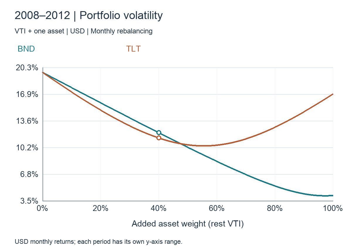
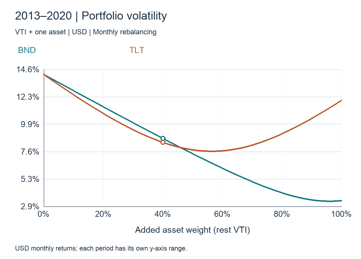
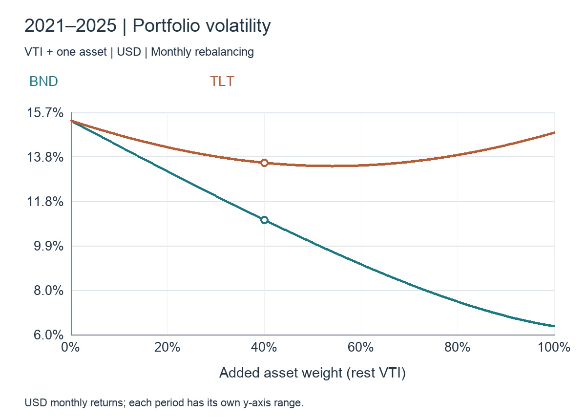
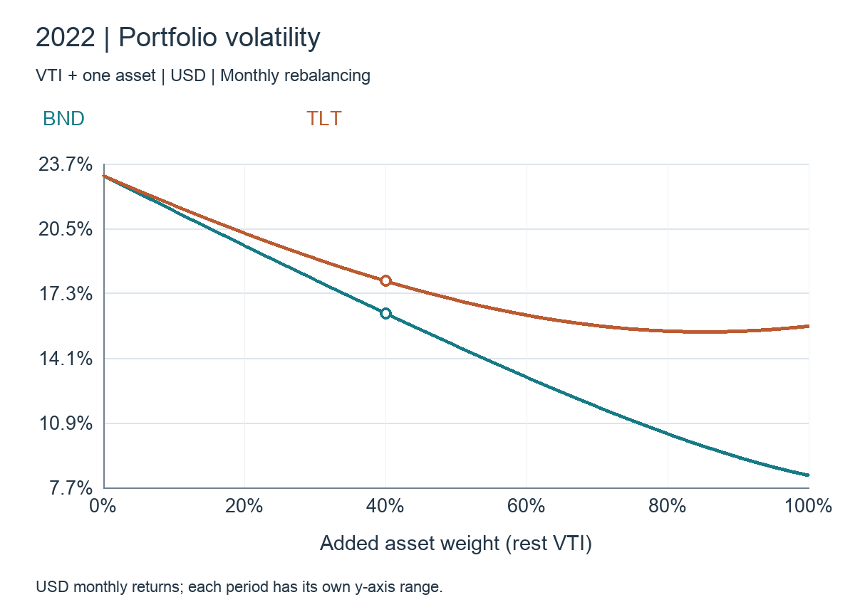
In 2013–2020, VTI’s annualized volatility was 14.18%; a 40% TLT allocation reduced it to 8.37%. In 2021–2025, the corresponding figures were 15.36% and 13.51%. Long bonds still reduced fluctuations, but offered far less offsetting power. Their own volatility was substantial and their correlation with equities had turned positive.
A 40% BND allocation reduced recent volatility to 11.02%. Even with positive correlation, replacing some equities with a less volatile asset reduces overall variation. That is different from diversification through opposite movements. Whether the lost return was worth the reduction in volatility is a separate question.
Return and Sharpe curves changed shape
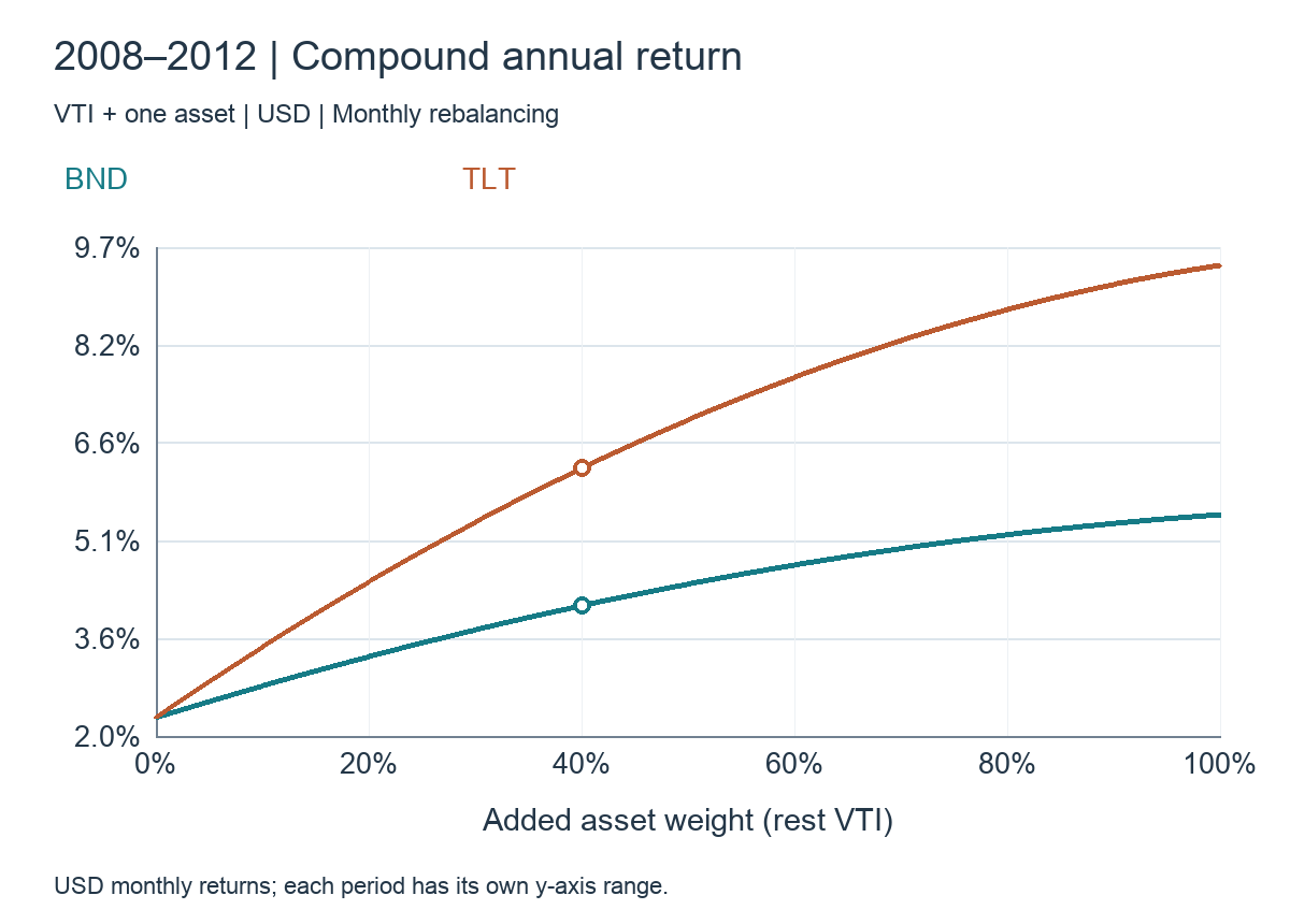
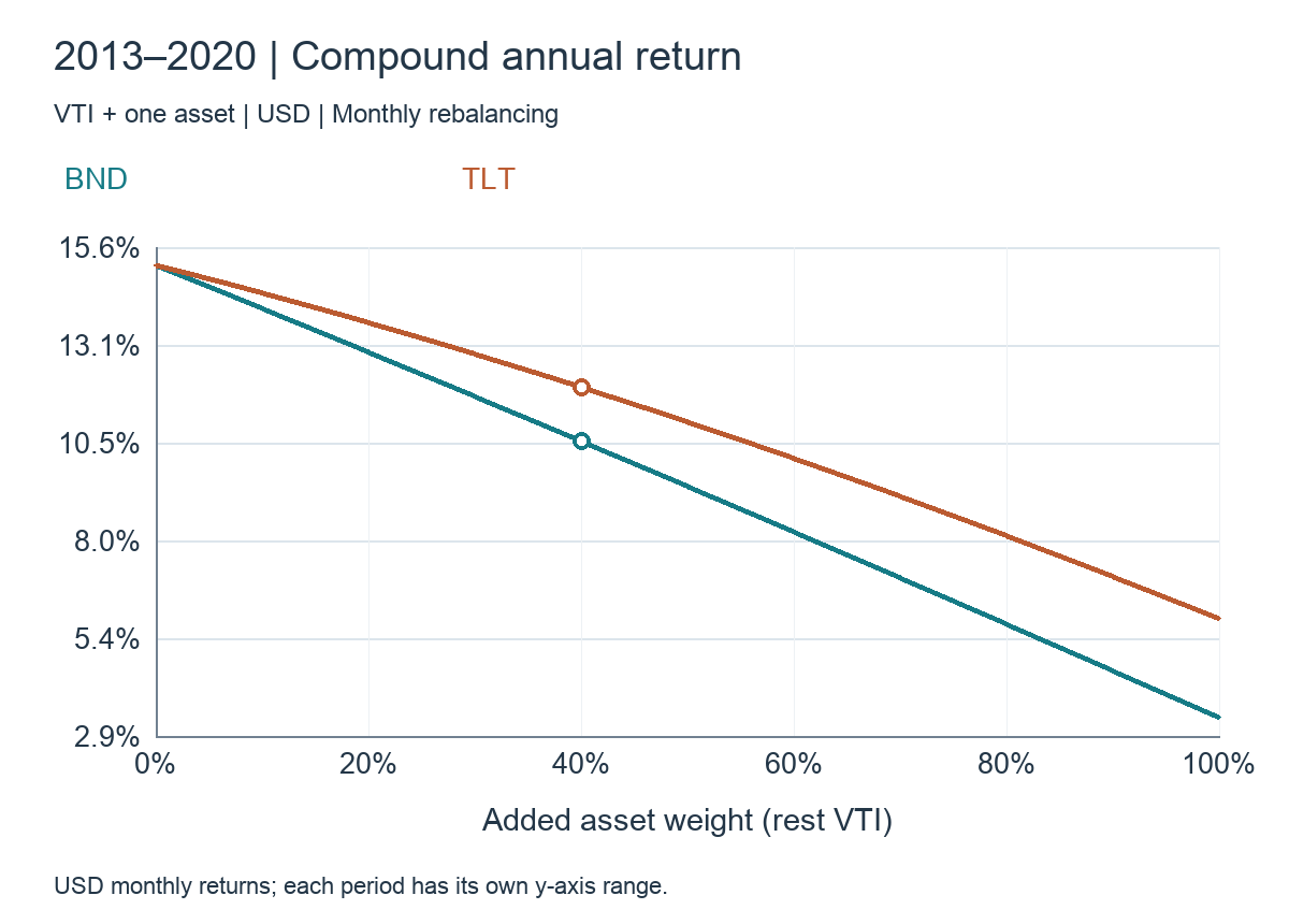
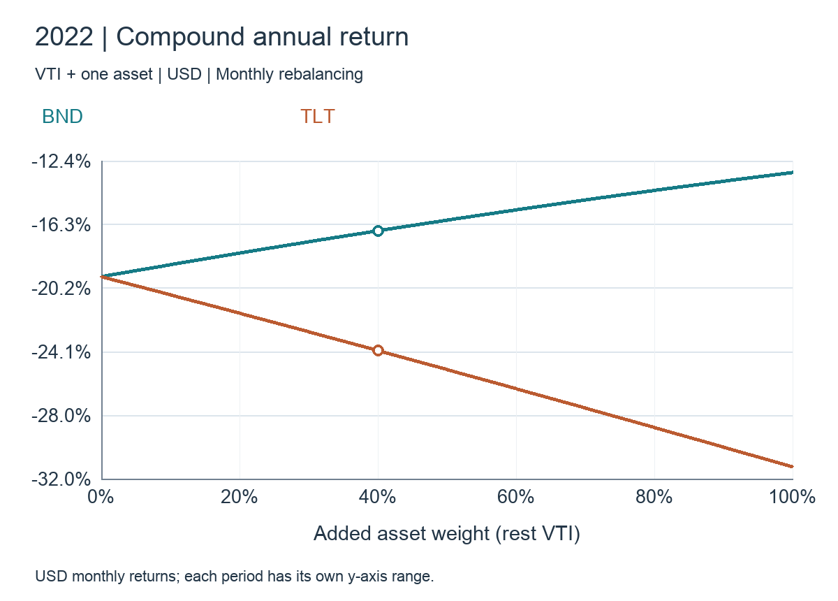
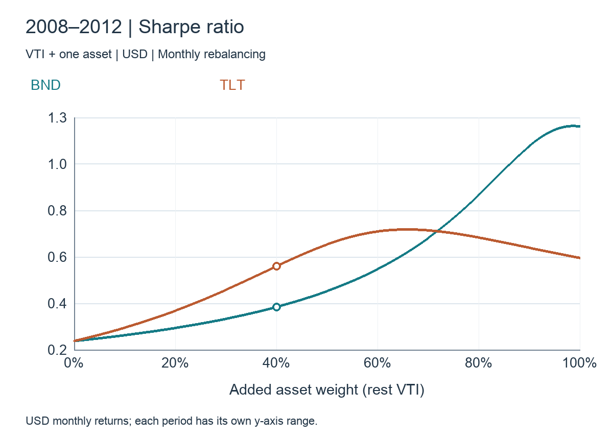
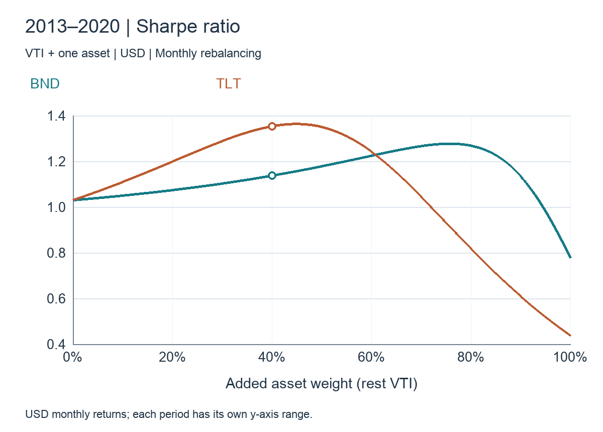
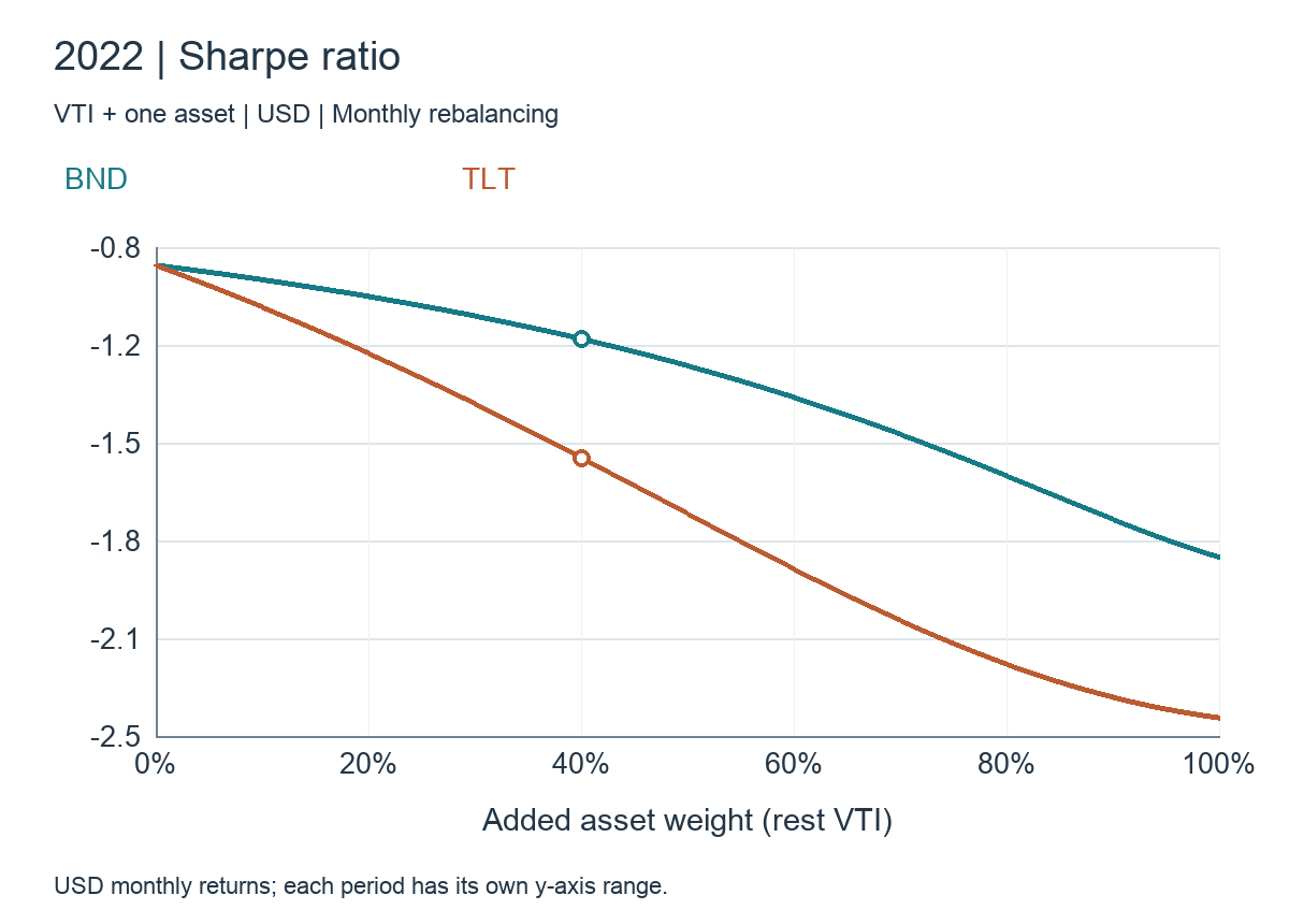
In 2013–2020, Sharpe ratios were 1.02 for VTI alone, 1.11 with 40% BND and 1.31 with 40% TLT. The reduction in variation more than compensated for the return given up. The TLT curve rises to an interior peak as bonds are added.
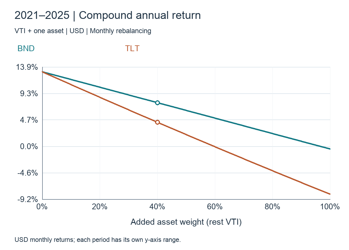
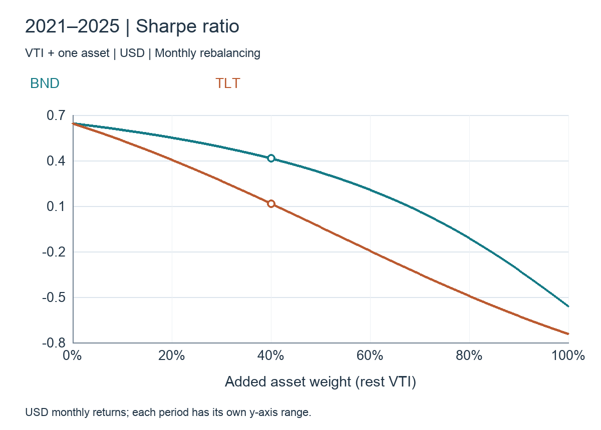
In 2021–2025, the corresponding ratios were 0.68, 0.44 and 0.14. For both bond choices, the maximum Sharpe in that sample occurred at a 0% bond weight. Annualized returns were 13.07%, 7.67% and 4.24%. Bonds reduced fluctuations somewhat, but reduced excess earnings much more.
Across the full 2008–2025 sample, both 60/40 portfolios had Sharpe ratios around 0.66, slightly above VTI’s 0.64. An improvement visible in the long aggregate disappears in the recent slice. Separating the crisis years, low-rate years and inflation years therefore matters. All 2022 Sharpe ratios are negative; read those numbers alongside returns and drawdowns rather than treating their ranking as a forward allocation recommendation.
Drawdowns expose the long-bond problem
| Period | Portfolio | Volatility | CAGR / return | Sharpe | Max drawdown |
|---|---|---|---|---|---|
| 2013–2020 | VTI | 14.18% | 15.15% | 1.02 | -20.82% |
| 2013–2020 | VTI 60% + BND 40% | 8.71% | 10.57% | 1.11 | -12.67% |
| 2013–2020 | VTI 60% + TLT 40% | 8.37% | 11.97% | 1.31 | -7.81% |
| 2021–2025 | VTI | 15.36% | 13.07% | 0.68 | -24.82% |
| 2021–2025 | VTI 60% + BND 40% | 11.02% | 7.67% | 0.44 | -20.66% |
| 2021–2025 | VTI 60% + TLT 40% | 13.51% | 4.24% | 0.14 | -26.74% |
| 2022 | VTI | 23.07% | -19.52% | -0.90 | -24.82% |
| 2022 | VTI 60% + BND 40% | 16.29% | -16.70% | -1.15 | -20.66% |
| 2022 | VTI 60% + TLT 40% | 17.88% | -24.07% | -1.54 | -26.74% |
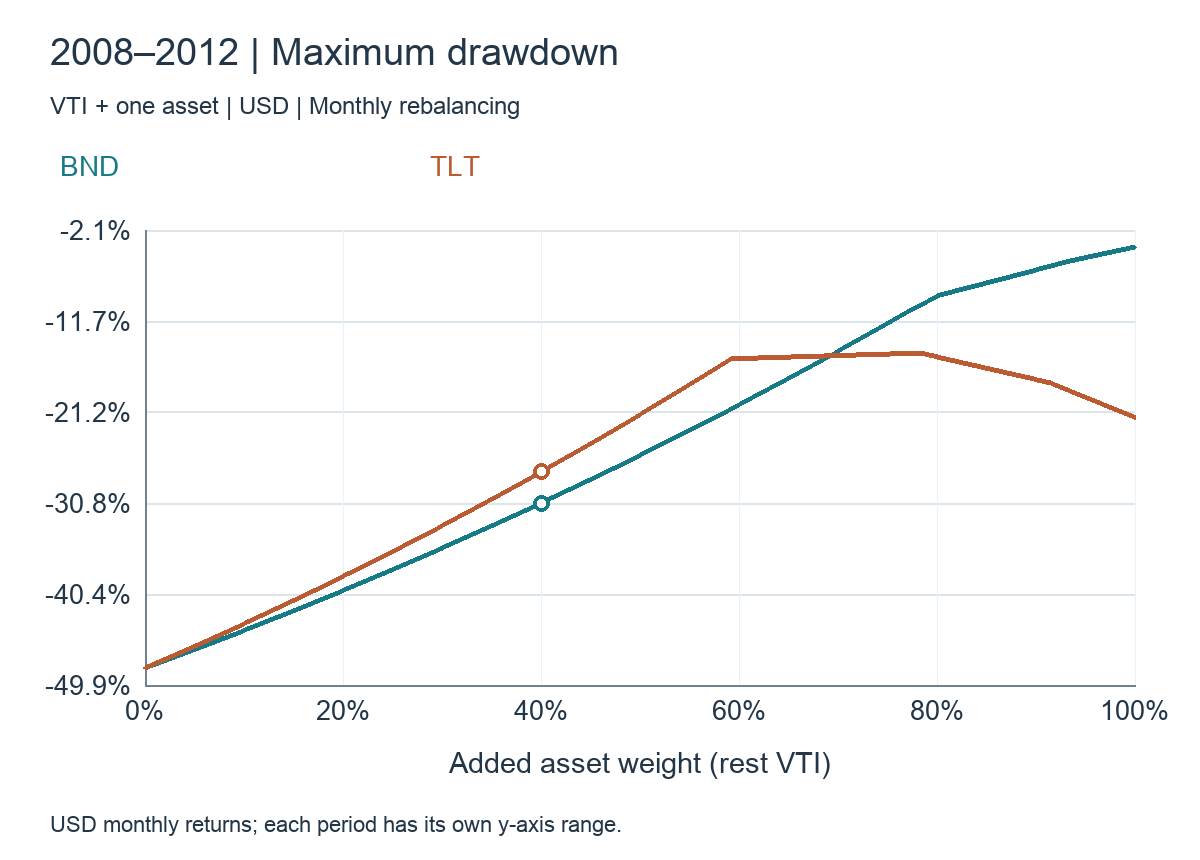
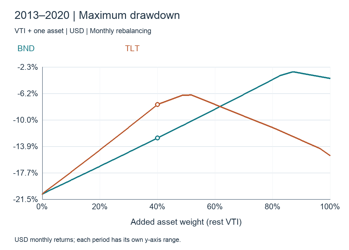
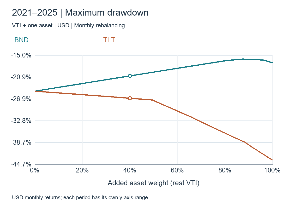
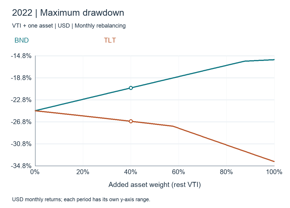
The 2021–2025 month-end maximum drawdowns were −24.82% for VTI, −20.66% with 40% BND and −26.74% with 40% TLT. BND retained some loss protection; TLT made the decline worse. In calendar 2022, VTI returned −19.52%, while the 60% VTI/40% TLT portfolio returned −24.07%.
Lower standard deviation does not guarantee a shallower maximum loss. Assets that decline together over an extended period can create a deeper drawdown despite smaller month-to-month variation. The result is not that all bonds failed on every measure. BND reduced both volatility and drawdown; TLT reduced volatility slightly but lost its drawdown protection. Neither improved recent Sharpe ratios.
Stay disciplined without ignoring the evidence
Replacing a disappointing allocation with the one that won the latest backtest is not a strategy for the next rate environment. After rates rise, bond income prospects change. Past capital losses and the income available from today’s yields are different considerations.
In its February 10, 2026 commentary, Vanguard explains that its time-varying 40% stock/60% bond model does not mean everyone should make a drastic allocation change. It is a risk/return signal for thinking about where the next dollar goes. Maintaining a strategy is not ignoring changing conditions. Set the allocation around spending needs, the investment horizon and tolerable losses, then maintain saving and rebalancing rules. Review from those objectives—not from the latest winner-and-loser table.
On this board, compare VTI, TLT and BND
Place TLT and BND beside VTI, and add the U.S. 10-year Treasury yield. Falling VTI and rising TLT reveal the offset associated with growth worries and lower yields. If both fall while yields rise, a common rate shock is a more useful interpretation. If BND falls less than TLT, differing interest-rate sensitivity matters more than declaring all bonds ineffective.
Also watch recoveries: do bonds rebound when equities do, and which asset regains its high first? Compare percentage changes and quote timestamps within the same U.S. session, not line heights. Daily board charts show price moves; this study includes reinvested distributions. Use aligned long-run returns to evaluate weights and the board to observe the forces operating today. Yen-based investors can add USD/JPY to separate the common currency exposure of U.S. holdings.
How the calculation works
Yahoo Finance daily distribution- and split-adjusted ETF prices were reduced to month ends. December 2007 supplies the starting level for 216 monthly returns from January 2008 through December 2025. There are no missing months or interpolated values. Bond weights run from 0% to 100% in 0.1-percentage-point steps, rebalanced monthly. Results are in USD without borrowing, taxes or trading costs; fund expenses are embedded in observed prices.
Monthly portfolio return is rₚ = (1−w)rVTI + w rbond. Volatility is sample monthly standard deviation × √12; annualized return is geometric CAGR. Sharpe subtracts the prior month’s FRED TB3MS ÷ 1200 as an approximate cash return, then uses mean monthly excess return ÷ its standard deviation × √12. Maximum drawdown includes starting wealth of 1 and measures losses from preceding month-end peaks—not intraday or daily losses. Each era starts afresh at 1. The twelve-month 2022 stress case also falls within 2021–2025. Data were retrieved and calculations completed on October 5, 2026.
Data and references
- Yahoo Finance — historical adjusted ETF prices: VTI, BND, TLT
- Federal Reserve / FRED — three-month Treasury bill rate
- Vanguard — BND
- iShares — TLT
- Harry Markowitz (1952) — Portfolio Selection
- Vanguard (2026-02-10) — Time to rethink your balanced portfolio’s next dollar