Stocks remain the core of long-term wealth building: companies earn profits, distribute cash and expand their businesses. Adding commodities has become much easier, however. Investors no longer need to store bullion at home or manage a futures account to place commodity exposure alongside equities. Listed funds and mutual funds provide practical access.
Which commodity makes the best partner? We compare VTI, the broad U.S. equity ETF, with investment vehicles representing the board’s seven commodities: gold, silver, copper, platinum, palladium, oil and natural gas. Across 2012–2025, gold produces both the lowest attainable portfolio volatility and the highest attainable Sharpe ratio. We examine fixed 20% allocations, full allocation curves and different eras to explain how it wins.
Commodity exposure fits inside a securities account
GLD and GLDM provide gold exposure, SLV silver, PPLT platinum and PALL palladium through physically backed trusts. CPER, USO and UNG use futures for copper, oil and natural gas. These listed products make commodity allocations operationally accessible alongside equities. Japanese investors also have the physical-backed Fruit of Gold series—1540, 1541, 1542 and 1543—and the Mitsubishi UFJ Gold Fund, which invests primarily in the gold trust.
Our comparison uses U.S.-listed products so all returns are in dollars and sampled on the same U.S. month-end sessions. GLD supplies a longer history than GLDM. VTI includes reinvested distributions. We use ETF as a convenient collective label, although precious-metal trusts and USCF commodity pools have legal structures different from conventional equity ETFs.
A commodity price chart is not a long-term investment return
Physically backed trusts reflect metal prices less expenses. Futures products also reflect contract rolls and collateral income. Contango and backwardation change the economics of maintaining exposure. The USO documentation describes futures, collateral interest and expenses; CPER selects copper contracts through index rules.
USO’s holdings changed during the 2020 dislocation, and CPER’s index rules also changed. We measure the products investors actually held through those changes, not an imaginary unchanging futures strategy. Split- and distribution-adjusted prices capture investable holding returns; simply joining front-month commodity prices would answer a different question.
Add 20%: gold stands out
| 20% partner / 80% VTI | Correlation with VTI | Annual volatility | CAGR | Sharpe |
|---|---|---|---|---|
| VTI 100% | — | 14.34% | 14.49% | 0.913 |
| Gold / GLD | +0.086 | 12.11% | 13.33% | 0.973 |
| Copper / CPER | +0.429 | 13.66% | 12.33% | 0.810 |
| Palladium / PALL | +0.174 | 13.73% | 13.55% | 0.885 |
| Platinum / PPLT | +0.364 | 13.82% | 12.35% | 0.804 |
| Silver / SLV | +0.254 | 14.03% | 13.52% | 0.870 |
| Oil / USO | +0.329 | 15.34% | 10.30% | 0.619 |
| Natural gas / UNG | +0.060 | 15.48% | 8.19% | 0.486 |
VTI alone has annualized volatility of 14.34%. Replacing 20% with gold reduces it to 12.11% and raises Sharpe from 0.913 to 0.973. CAGR declines from 14.49% to 13.33%. This is not return maximization: lower fluctuations improve the amount of historical reward earned per unit of risk.
At the same 20% allocation, copper delivers 13.66% volatility, palladium 13.73%, platinum 13.82% and silver 14.03%. Industrial-metal exposure does not automatically create strong equity diversification.
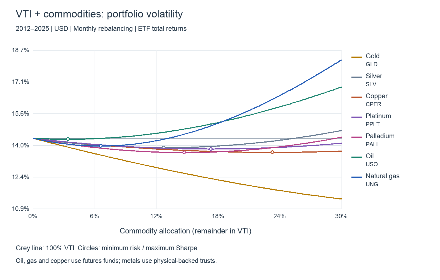
Natural gas has a lower equity correlation than gold: +0.060 against +0.086. Yet a 20% gas allocation increases portfolio volatility to 15.48%, because UNG itself has 48.60% annualized volatility. Oil at 20% also increases volatility, to 15.34%. A different return pattern is not enough: the size of the partner’s own fluctuations matters.
Correlation and standalone volatility work together
Portfolio variance is σPF² = (1−w)²σstocks² + w²σcommodity² + 2w(1−w)ρσstocksσcommodity. Lower correlation reduces the interaction term, but high commodity volatility makes the second term grow rapidly as the allocation increases.
Standalone annualized volatility is 15.05% for gold, 19.90% for copper, 22.99% for platinum, 28.39% for silver, 29.04% for palladium, 35.47% for oil and 48.60% for gas. Gold combines low equity correlation with volatility close to stocks. That combination drives its deeper diversification benefit.
Minimum risk and maximum Sharpe are different allocations
| Partner | Min-risk weight | Min volatility | Max-Sharpe weight | Peak Sharpe |
|---|---|---|---|---|
| Gold / GLD | 47.3% | 10.82% | 28.1% | 0.981 |
| Palladium / PALL | 14.7% | 13.64% | 7.0% | 0.922 |
| Copper / CPER | 23.3% | 13.64% | 0.0% | 0.913 |
| Platinum / PPLT | 17.3% | 13.81% | 0.0% | 0.913 |
| Silver / SLV | 12.7% | 13.88% | 4.3% | 0.916 |
| Natural gas / UNG | 6.6% | 13.96% | 0.0% | 0.913 |
| Oil / USO | 3.4% | 14.29% | 0.0% | 0.913 |
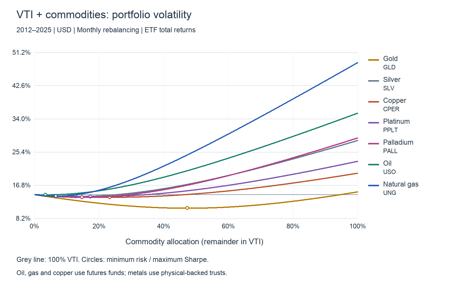
Gold reaches minimum portfolio volatility at 47.3%, producing 10.82% volatility—about 24.5% below VTI’s 14.34%. Its maximum-Sharpe allocation is instead 28.1%, with a Sharpe of 0.981. The remaining 71.9% equity allocation preserves more of the sample’s stock returns while retaining gold’s diversification.
These exact weights describe the historical curves, not forward allocation instructions. My starting point for an equity-centered portfolio is to examine gold in the 10–20% range and choose a weight that is practical to maintain. In this sample, 10% gold produces 13.12% volatility and 20% produces 12.11%; diversification does not require chasing the exact minimum.
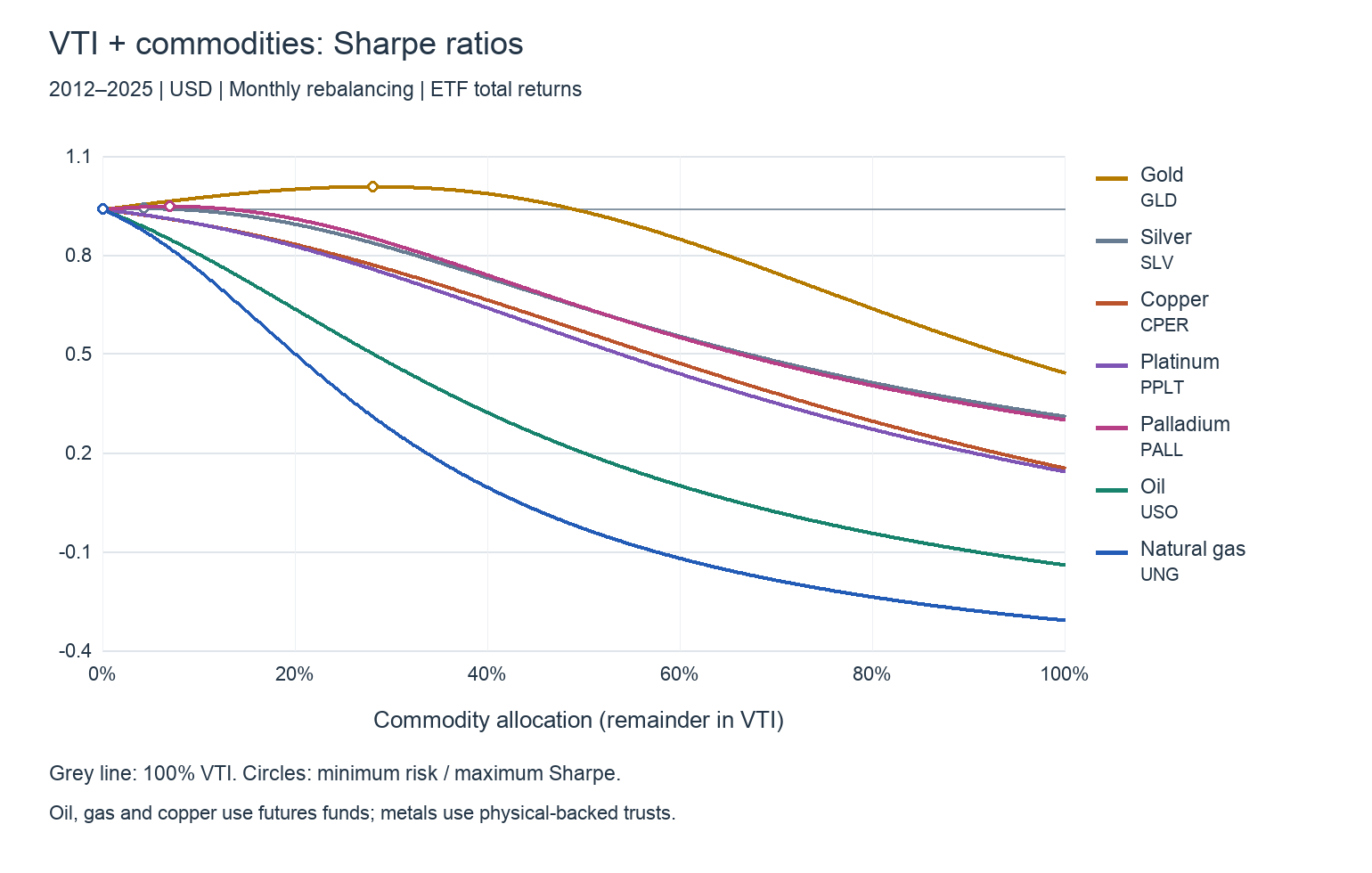
The highest full-sample Sharpe ratios across the separate commodity portfolios are gold’s 0.981, palladium’s 0.922 and silver’s 0.916. Copper, platinum, oil and gas each maximize Sharpe at a zero commodity allocation: VTI alone. The small improvements for palladium and silver are not equivalent to gold’s larger improvement. Selecting tiny historical wins from many alternatives provides a weak foundation for forward allocation.
Separate the eras: risk reduction persists, return efficiency changes
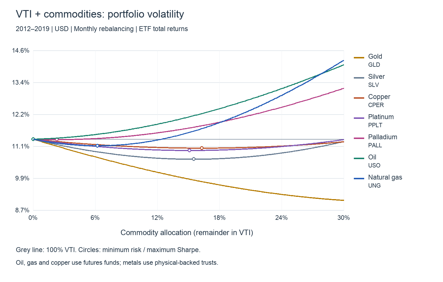
2012–2019
| Portfolio | Annual volatility | Sharpe |
|---|---|---|
| VTI 100% | 11.31% | 1.207 |
| Gold 20% | 9.51% | 1.142 |
| Silver 20% | 10.64% | 0.955 |
| Copper 20% | 11.00% | 0.933 |
| Oil 20% | 12.65% | 0.707 |
| Natural gas 20% | 12.21% | 0.630 |
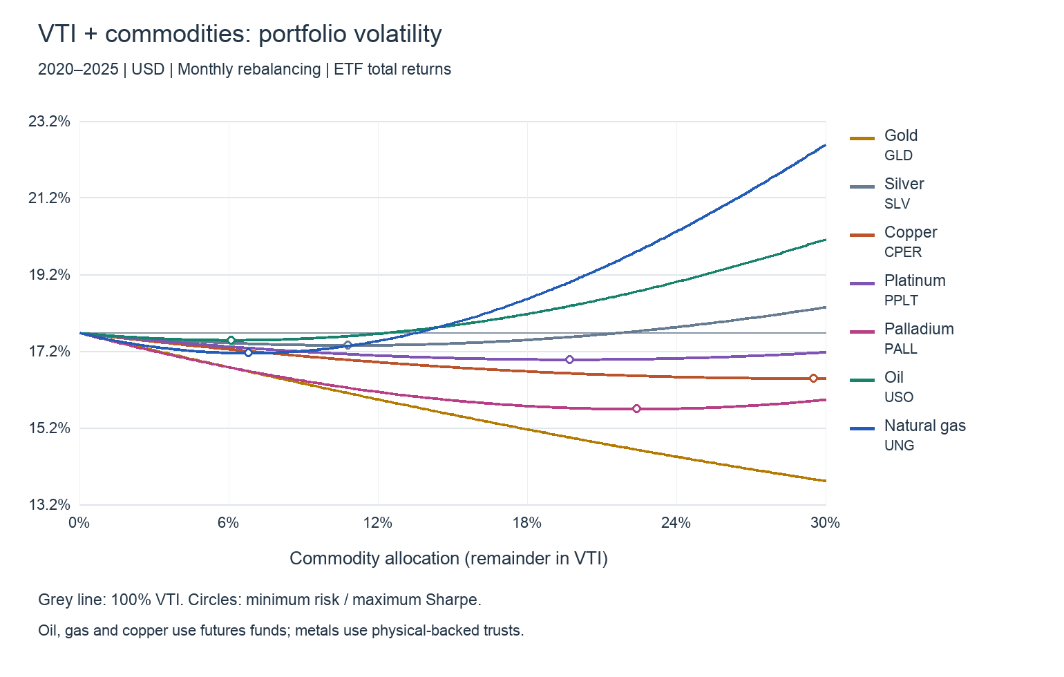
2020–2025
| Portfolio | Annual volatility | Sharpe |
|---|---|---|
| VTI 100% | 17.67% | 0.698 |
| Gold 20% | 14.93% | 0.869 |
| Silver 20% | 17.58% | 0.846 |
| Copper 20% | 16.62% | 0.729 |
| Oil 20% | 18.41% | 0.555 |
| Natural gas 20% | 19.07% | 0.384 |
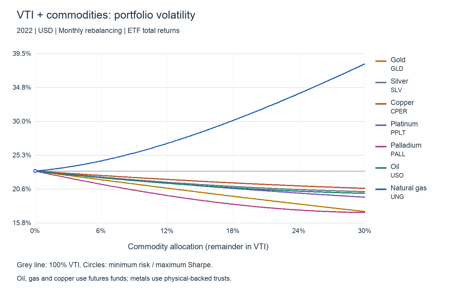
2022
| Portfolio | Annual volatility | Sharpe |
|---|---|---|
| VTI 100% | 23.07% | -0.903 |
| Gold 20% | 19.18% | -0.887 |
| Silver 20% | 20.76% | -0.765 |
| Copper 20% | 21.27% | -0.932 |
| Oil 20% | 20.55% | -0.539 |
| Natural gas 20% | 31.33% | -0.196 |
In 2012–2019, 20% gold reduces volatility from 11.31% to 9.51%, but Sharpe falls from 1.207 to 1.142. Gold diversifies the fluctuations while its lower returns reduce historical reward per unit of risk.
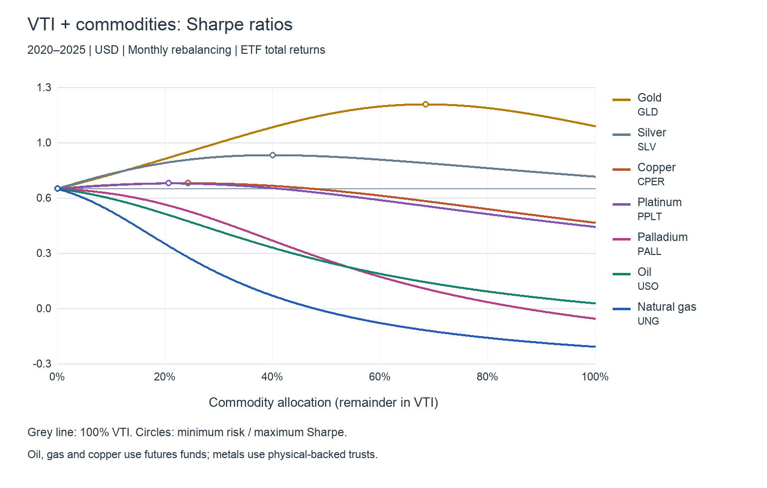
In 2020–2025, 20% gold reduces volatility to 14.93% and raises Sharpe from 0.698 to 0.869. The recent period’s maximum-Sharpe gold weight is 68.5%, far above the full-sample 28.1%. The direction of risk reduction survives both eras; the allocation that earned the highest historical Sharpe changes dramatically.
2022 illustrates another regime. USO returns +28.97%, while VTI loses 19.52%. A 20% oil allocation reduces annual volatility to 20.55%, versus 23.07% for VTI. Yet oil at 20% increases risk over the full sample. Strength during an inflation and supply-stress year is different from being a reliable long-run portfolio stabilizer.
For forward decisions, emphasize portfolio risk rather than backtested returns
Historical returns can be measured accurately as outcomes. They should not simply be relabeled expected future returns. MIT’s investment lecture notes explain both the difficulty of estimating expected returns and the extreme sensitivity of optimized weights to return assumptions. Merton’s research argues that adding historical excess returns to current interest rates fails to account for changing market risk.
Even in a simple independent, constant-distribution model, the standard error of an annualized mean is approximately σ/√T. Using 14.34% volatility and 14 years gives roughly 3.83 percentage points. Small apparent advantages in historical average returns sit inside substantial estimation noise.
Volatility and correlation describe the structure of fluctuations and co-movement. They can be easier to estimate than means and offer useful inputs for allocation design. They still change with crises and product structures, so examine different eras rather than treating one covariance matrix as permanent. That is why we test whether gold’s volatility reduction appears in both halves of the sample.
My conclusion is to emphasize risk reduction that appears across multiple periods, rather than chase the best historical return or Sharpe ranking. Sharpe evaluates the efficiency of the realized past; it does not determine future expected returns. Minimum variance alone can also remove too much equity exposure. Decide first how central equities should remain and what allocation is sustainable.
Use the board to study days when the assets disagree
Place VTI beside gold and add silver or oil. Does gold hold up on an equity sell-off? Does silver swing more sharply despite moving with gold? Oil strength alongside equity weakness is a starting point for examining supply-side news rather than assuming stronger demand.
Copper moving with stocks invites investigation of shared manufacturing and economic-demand drivers. Gas moving alone invites a closer look at weather and inventories. Assets do not need to move in opposite directions every day. Diversification comes from imperfect long-run co-movement and a partner whose own fluctuations do not overwhelm the portfolio.
Use percentage changes and percentage reference lines, not visual slopes. VTI follows a U.S. equity session while commodity charts use different windows; match the periods you compare. Daily observation should improve understanding of the holdings, not trigger a new allocation after every unusual day.
Data and calculation
The starting observation is the final U.S. session of December 2011, followed by 168 monthly returns from January 2012 through December 2025. We use Yahoo Finance adjusted daily closes for VTI, GLD, SLV, CPER, PPLT, PALL, USO and UNG. All products must have actual observations on VTI’s final session of each month; missing values are not filled. The common window accommodates CPER’s inception.
Each test is a separate VTI/one-commodity portfolio rebalanced monthly to constant weights. No leverage or shorting; commodity weights range from 0–100% in 0.1 percentage-point steps. Annual volatility is sample monthly-return standard deviation multiplied by √12. Sharpe is mean monthly excess return divided by its sample standard deviation, multiplied by √12. The risk-free proxy is the previous month’s FRED TB3MS annual percentage yield divided by 1200. CAGR is geometric growth from the monthly wealth series.
Fund expenses, actual rolls and collateral management are embedded in prices. Personal taxes, trading commissions and currency conversion are excluded. This is a USD comparison, not the return of a yen-denominated investment. The 2022 stress case overlaps the recent period. Optimal points use each entire period retrospectively and are not forecasts or forward-tested trading strategies. Calculated October 14, 2026.
Data and references
- Vanguard — VTI
- SPDR — GLD / GLDM
- iShares — SLV
- Aberdeen — PPLT
- Aberdeen — PALL fact sheet
- USCF — CPER
- USCF — USO
- USCF — UNG
- 三菱UFJ信託銀行 — 金の果実 / Fruit of Gold
- 三菱UFJアセットマネジメント — 純金ファンド / Gold Fund
- MIT OpenCourseWare — Expected-return estimation and optimization sensitivity
- Merton (1980) — On Estimating the Expected Return on the Market
- FRED — TB3MS
- Yahoo Finance — VTI historical prices
- Yahoo Finance — GLD historical prices
- Yahoo Finance — SLV historical prices
- Yahoo Finance — CPER historical prices
- Yahoo Finance — PPLT historical prices
- Yahoo Finance — PALL historical prices
- Yahoo Finance — USO historical prices
- Yahoo Finance — UNG historical prices