Experienced investors often start with the losses they can withstand, rather than the return they hope to earn. A disappointing gain can be tolerated; a forced sale to meet spending or debt obligations can end an investment plan.
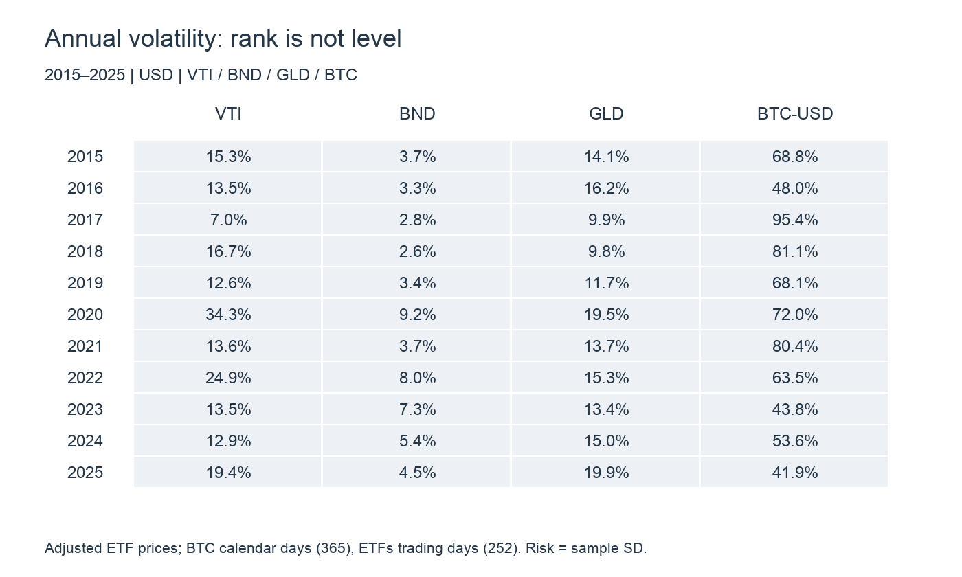
Our 2015–2025 comparison finds a clear distinction. Across US equities, aggregate bonds, gold and bitcoin, average adjacent-year rank correlation was −0.06 for annual returns and 0.90 for volatility. Yet US equity volatility ranged from roughly 7% to 34%. Relative risk persisted; its numerical level did not stay constant.
Three examples of putting risk first
Howard Marks’s Oaktree puts risk control first in its investment philosophy. Good-market gains alone do not establish skill; performance in difficult markets helps reveal the risk taken to earn them. This is not indifference to returns, but attention to how they are earned. Oaktree’s philosophy
Ray Dalio’s Bridgewater describes All Weather through risk balancing. Equal dollars in stocks and bonds need not create equal risk: equities can dominate portfolio fluctuations. The approach starts with exposure to growth and inflation rather than assuming capital weights measure diversification. The All Weather Story
Warren Buffett adds an important distinction. His 2014 shareholder letter rejects treating volatility as synonymous with risk and emphasizes purchasing power and investment horizon. Funds needed soon require different treatment from capital invested for decades. Permanent loss, liquidity needs and forced selling are risks that standard deviation alone does not capture. Berkshire’s 2014 letter, printed page 18
Separate realized return from realized volatility
Here, “risk” means annualized standard deviation of daily returns, not bankruptcy probability or maximum drawdown. Everything is measured in US dollars, without yen conversion.
| Exposure | Instrument | What it represents |
|---|---|---|
| US equities | VTI | Broad US stock ETF |
| US bonds | BND | Investment-grade aggregate bonds, not cash |
| Gold | GLD | Gold trust shares, net of fund expenses |
| Bitcoin | BTC-USD | Spot USD daily prices, including weekends |
ETF prices are adjusted for distributions and splits; bitcoin uses spot prices. GLD represents an investable gold exposure, not the identical price series used by this board’s gold chart.
Return winners change
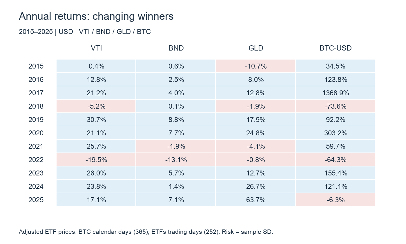
Bitcoin gained approximately 1,369% in 2017 but lost about 64% in 2022. Gold lost roughly 0.8% in 2022 and gained about 64% in 2025. Equity and bond results also changed with growth and interest-rate conditions. Last year’s winner is not automatically next year’s opportunity.
Risk rankings persist more than risk levels
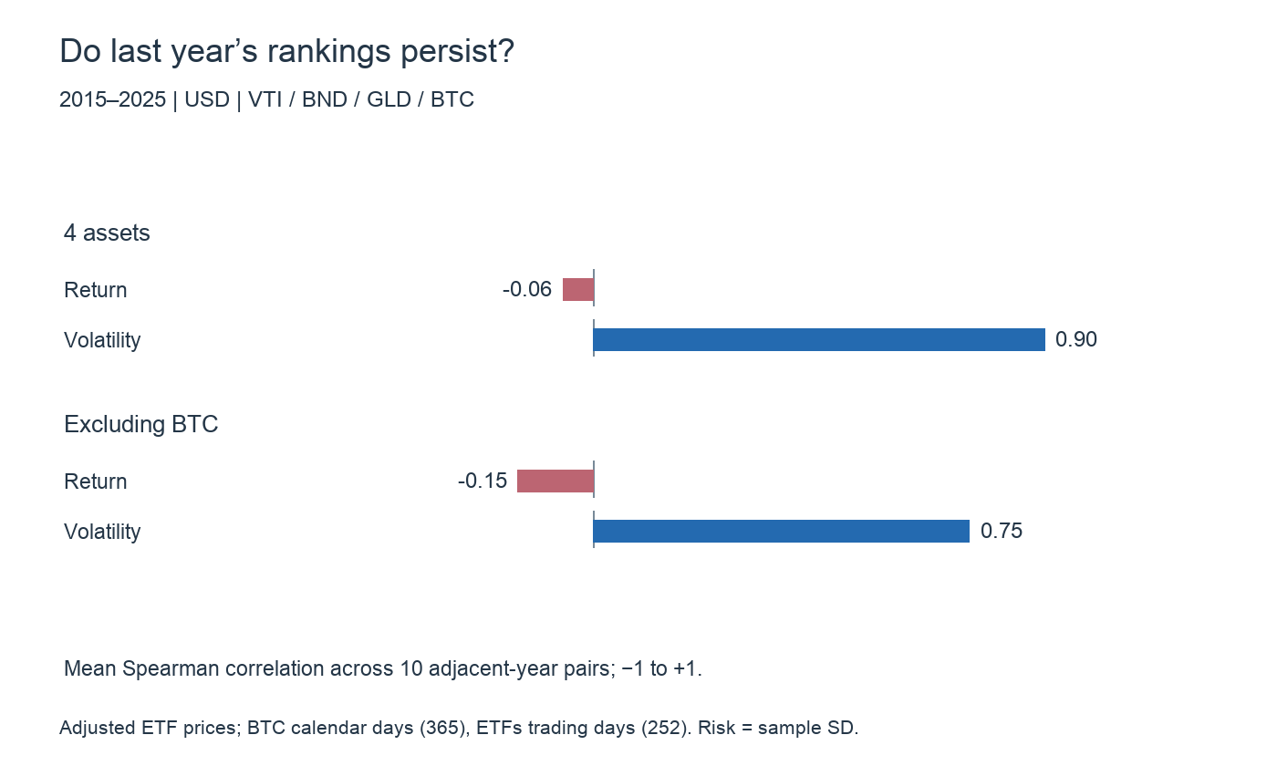
| Sample | Return rank | Risk rank |
|---|---|---|
| Four assets | -0.06 | 0.90 |
| Excluding BTC | -0.15 | 0.75 |
For each year, rank the assets and compare that order with the following year using Spearman correlation: +1 means identical order, −1 reversed order, and near zero little rank association. The table averages ten adjacent-year pairs, from 2015–2016 through 2024–2025.
Bitcoin’s distinctive risk could make the comparison too easy, so we also remove it. Among the remaining three assets, average return-rank correlation is −0.15 and volatility-rank correlation 0.75. This supports relative risk persistence in this sample, not a claim about all assets or closely related stocks. Four assets and ten year pairs are a small descriptive comparison.
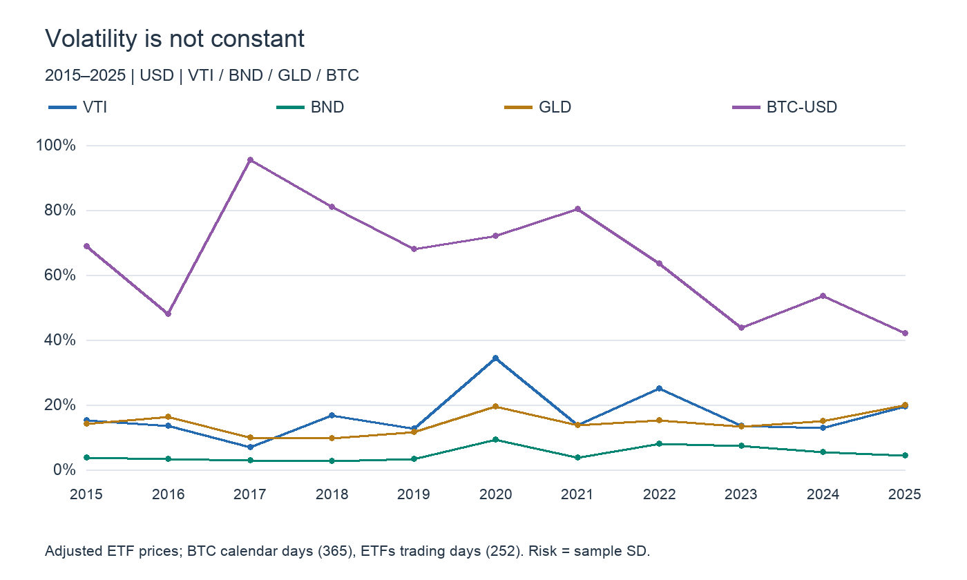
VTI volatility rose from 6.99% in 2017 to 34.28% in 2020. BND reached 9.23% in 2020. Bonds remained less volatile than equities in this sample, but were not equally calm every year. BND’s −13.11% return in 2022 also shows that low standard deviation is not protection against a sustained loss.
How wrong is a simple prior-year forecast?
| Asset | Lowest risk | Highest risk | Prior-year forecast MAE |
|---|---|---|---|
| VTI | 6.99% | 34.28% | 9.43 pp |
| BND | 2.64% | 9.23% | 2.10 pp |
| GLD | 9.75% | 19.85% | 3.40 pp |
| BTC-USD | 41.92% | 95.37% | 16.58 pp |
Predict each year’s volatility using only the previous year’s realized volatility. The mean absolute error across 2016–2025 is 9.43 percentage points for VTI. A 10% forecast versus 20% realized volatility is a ten-point error. Stable rankings and accurate numerical forecasts are different achievements.
Why estimating volatility can be easier than estimating mean returns
Daily returns contain persistent expected compensation plus large positive and negative surprises. Estimating the mean requires extracting a small signal from that noise. Variance instead aggregates squared deviations, which do not cancel.
Consider a textbook model with constant mean and variance, independent normally distributed daily returns and 20% annual volatility. Even ten years give an approximate standard error of 20% divided by √10, or 6.3 percentage points, for the annualized arithmetic mean. Dividing the same ten years into more frequent observations does not create more independent years. The difficulty of estimating expected returns is central to Merton (1980).
With approximately 2,520 observations under those same ideal assumptions, the approximate standard error of estimated annual volatility is 20% divided by √(2×2,519), or 0.28 percentage points. This compares estimation of constant parameters, not the accuracy of next year’s volatility forecast. Fat tails, dependence and changing variance make real-world uncertainty more complicated.
Risk changes, but its changes have persistence
Large moves tend to cluster together, as do quiet periods. Engle’s 1982 ARCH framework modeled changing variance using past shocks. The useful insight is not that volatility is constant, but that its dynamics contain information. Engle’s Nobel lecture / What Good Is a Volatility Model?
Interest-rate sensitivity, business models, leverage and market participation also persist, helping preserve differences across assets. Crises and structural changes can nevertheless break historical levels. Our annual ranking exercise does not test ARCH or establish short-horizon forecast accuracy.
Use the board to compare behavior, not just gains
Compare VTI, BND, gold and BTC over multiple days using percentage changes, not dollar changes or the visual height of differently scaled lines. Add VIX to distinguish realized volatility from option-implied expectations for roughly the next 30 days of the S&P500.
A daily percentage change is an endpoint comparison, not the total amount of intraday movement. Bitcoin’s rolling 24-hour window also differs from the US ETF session. Use long-run statistics to size exposure and the board to notice changing conditions; a single day cannot establish annual risk.
Calculation details
Eleven calendar years, January 2015–December 2025. ETF simple daily returns use adjusted trading-day closes; BTC uses calendar-day spot returns including weekends. Annual return is the product of (1+r) minus one. Annual volatility is sample standard deviation (n−1 denominator) multiplied by √252 for ETFs and √365 for BTC. Include the return from the previous year’s last observation into the first observation of the year. No holiday filling or removal of BTC weekends. Annual statistics therefore use each asset’s native calendar. No tax, transaction costs or currency conversion. Recalculated from previously cached public price histories. These current representative assets do not cover the entire investment universe. Cross-sectional rank persistence is not proof of return predictability.
Data and references
- Oaktree: Investment Philosophy
- Bridgewater: The All Weather Story
- Berkshire Hathaway: 2014 shareholder letter, p.18
- Merton (1980): On Estimating the Expected Return on the Market
- Engle (2003): Nobel Lecture
- Engle (2000): What Good Is a Volatility Model?
- Yahoo Finance: adjusted ETF and BTC daily price histories