Edward Oakley Thorp was born in Chicago on August 14, 1932. He studied physics at UCLA, earned his mathematics doctorate there in 1958, and taught at MIT and New Mexico State before joining the founding faculty of UC Irvine in 1965. His route to investing began in a mathematics department, not a brokerage.
He would overturn conventional thinking about blackjack and build an investment business around relationships between security prices. Two questions explain his approach better than a talent for forecasting: What should this security cost, and what can I combine with it to reduce the risks I do not want?
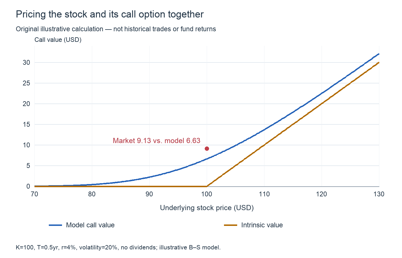
The chart is our own calculation of a stock and the right to buy it at a fixed price. When the market quote departs from a model curve, an investor can investigate an offsetting stock-and-option position. Below, we work through the numbers rather than treating the gap as guaranteed profit.
A mathematician whose work extended beyond cards
Thorp worked in functional analysis, linear operators, normed spaces, probability, statistics and game theory. Functional analysis studies spaces of functions and the transformations acting on them. His practical interests did not replace this abstract mathematical work.
In his 2003 account, he explained how linear approximations familiar from functional analysis helped simplify the enormous space of depleted card decks. At MIT he used an IBM 704 to do the calculations. Recognize a structure, reduce the problem, and test it computationally: the method carried over to finance. Thorp's account
Blackjack: earlier cards change the next round's conditions
A run of red results does not make black more likely on an ordinary independent roulette spin. Blackjack is different: cards already dealt are not necessarily returned and shuffled after every round. The composition of the remaining deck changes, so the conditions for the next round change too.
Thorp studied this sampling without replacement. The remaining mix of high cards and aces can alter the player's expectation. Tracking exposed cards and changing the amount at risk links conditional probability to position size; it is not simply an exercise in memory.
His 1961 paper, A Favorable Strategy for Twenty-One, preceded Beat the Dealer in 1962. The achievement was not a promise to win every hand. It showed how particular rules and deck compositions could create a positive expectation over repeated play. The original paper
He also worked with information theorist Claude Shannon on a small wearable computer to predict roulette outcomes from physical measurements. In one problem the useful observation was the deck composition; in the other it was motion. Both approaches brought measurable information to activities commonly described as luck. Official biography
From forecasting stocks to pricing related securities
Economist Sheen Kassouf became his collaborator. Their 1967 book Beat the Market examined warrants and the underlying common shares. A warrant grants a right to purchase shares on specified terms. Because the warrant and stock generally respond together to the stock price, an offsetting long and short position can reduce exposure to the direction of the market.
In November 1969 Thorp and Jay Regan launched Convertible Hedge Associates, later renamed Princeton/Newport Partners, or PNP. The business expanded across warrants, over-the-counter options and convertible securities. Its distinction was systematic valuation combined with hedging, not simply participating in a rising stock market. Thorp's retrospective
What did he know before Black and Scholes?
The familiar claim that Thorp anticipated Black-Scholes needs a clear chronology. Finding a useful trading formula and publishing a proof of a general pricing theory are different achievements.
- The 1965–1967 work and book. Stock-and-warrant hedging ideas were public before 1973. The existence of the 1967 book does not, on its own, establish that the later pricing formula had already been fully proved.
- His account of 1967–1968. In a retrospective published in 2001, Thorp described setting both the stock's growth rate and the discount rate equal to the risk-free rate. That leads to the form of the later Black-Scholes formula. The dating here is his retrospective testimony.
- The 1973 paper and later explanation. He presented Extensions of the Black-Scholes Option Model in August 1973. In the 2018 AQR interview, he explained that his formula and Black's matched once differences in the treatment of short-sale proceeds were aligned.
Together these sources support the account that he independently developed and used pricing ideas before the landmark 1973 Black-Scholes paper. They do not require us to transfer credit for its published general theory to him. His achievement included making valuation work under the financing conditions of actual trades. His 2001 retrospective / His 1973 paper / AQR interview
A numerical trade: sell the expensive right, hedge with stock
This is an explanatory calculation, not a reconstruction of one of Thorp's orders. Assume a stock at $100 and a European call with a $100 strike and six months remaining. The continuously compounded annual risk-free rate is 4%, volatility is 20%, and there are no dividends. The Black-Scholes call value is $6.63.
Now suppose the market quote is $9.13, or $2.50 above model value. Selling the call alone exposes the seller to potentially large losses if the stock rises. Buying stock alongside the sale can offset part of that exposure.
Delta determines the initial hedge. It measures the change in option value for a small change in the underlying stock price. Here delta is about 0.584: sell one option unit and buy approximately 0.584 shares. A small stock rise produces a gain on the shares that approximately offsets the loss on the short option. For a 100-share contract, the corresponding stock hedge is about 58.4 shares.
The two sides are not equal dollar amounts. They are matched sensitivities. Delta changes with the stock price and remaining time, so maintaining the hedge requires changes in share holdings. The ratio and its adjustment are part of the trade, not an afterthought.
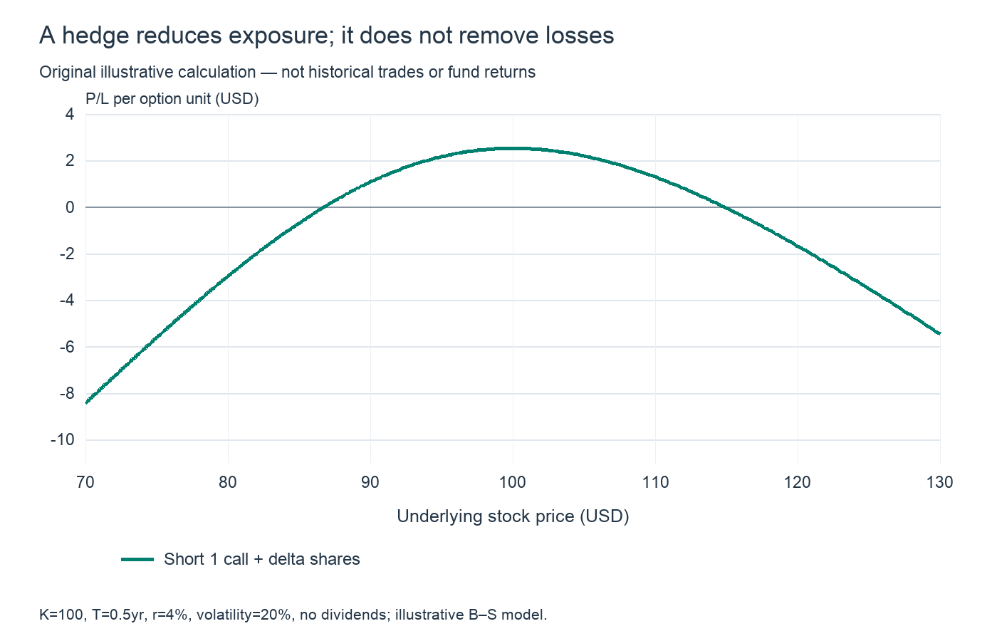
For this chart we keep the initial share position unchanged for one trading day and assume the entire overpricing disappears then. Time advances by 1/252 of a year, volatility remains 20%, and interest is charged on the net funds needed to establish the position.
| Stock after one day | Hedged P/L per unit |
|---|---|
| $80 | $-2.98 |
| $95 | $+2.16 |
| $100 | $+2.52 |
| $105 | $+2.19 |
| $120 | $-1.68 |
P/L is relatively stable between stock prices of $95 and $105, but becomes negative at $80 and $120. Initial delta offsets local, first-order sensitivity, not arbitrary changes in price. Rebalancing, jumps, changes in volatility, stock-borrow charges and bid–ask spreads all affect realized results. Market-neutral does not mean loss-free.
The chart also assumes convergence after one day. In a real trade the discrepancy can persist or widen. The $2.50 is a model-implied price difference, not profit secured when the sale is executed. The task is to collect it after the costs and risks of the hedge.
Convertible bonds and statistical arbitrage
A convertible bond combines a bond's payments with the right to convert into shares. Thorp modeled the straight-bond component separately from the conversion privilege. An underpriced convertible could be bought while stock was sold to reduce stock-price sensitivity. Credit quality, interest rates and stock-borrow conditions matter alongside the underlying share price.
He later pursued statistical arbitrage across baskets of shares. A stock and its warrant have a contractual relationship; two stocks have an estimated statistical relationship. These are not interchangeable foundations. A historical relationship between two stock-price series can break, so a widening visual gap alone does not establish a convergence trade.
The record: strong returns with unusually few losing months
The introduction to Thorp's 2017 Chat With Traders interview reports an approximately 19-year annualized PNP return of 19.1% before fees, 227 profitable months out of 230, and a worst monthly loss below 1%. The positive-month proportion is about 98.7%, calculated as 227/230. That is a fund-level monthly statistic, not the win rate of individual trades. Interview and reported performance
We do not turn this summary into an invented smooth wealth curve. A pre-fee statistic is also not the investor's net return. What matters for this account is the longevity of a hedged process whose results were not meant to depend solely on market appreciation. PNP moved into liquidation in 1988; Thorp's investment work continued through other activities.
The Kelly criterion: an edge does not justify unlimited size
Thorp researched and applied the Kelly criterion, named for John L. Kelly. Its objective is expected logarithmic wealth, rather than the largest expected dollar profit. That distinction puts compounded growth and position size at the center of the decision. The Kelly Criterion and the Stock Market
Consider an independent binary model with known win probability p. A win earns the amount risked; a loss loses it. Risking fraction f of current capital each round gives expected log growth g(f)=p log(1+f)+(1−p) log(1−f). In this particular model the maximizing fraction is f*=2p−1.
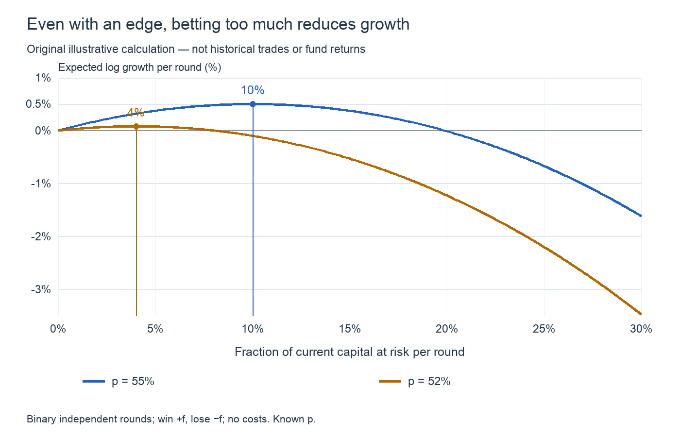
| Fraction f | Growth if p=55% | Growth if p=52% |
|---|---|---|
| 4% | +0.320% | +0.080% |
| 5% | +0.375% | +0.075% |
| 10% | +0.501% | -0.101% |
| 20% | -0.014% | -1.230% |
| 30% | -1.620% | -3.477% |
At p=55%, the optimum is 10%. At p=52%, it is only 4%. If you assume 55% and risk 10% each time, but the real probability is 52%, expected log growth is negative. A modest error in the estimated edge can turn a seemingly sensible position into overbetting.
These are per-round expected logarithmic growth rates, not annual returns or real blackjack win probabilities. Thorp and co-authors also studied full and fractional Kelly strategies: full Kelly can produce large short- and medium-term fluctuations, while reducing the fraction trades some growth for lower risk. It is not a license to feed historical stock returns into a formula and borrow the resulting amount tomorrow. Research on full and fractional Kelly
Why a market-beater recommends index funds
Thorp argues for low-cost indexing when an investment cannot be shown to improve on a comparable index. A market may contain inefficiencies without giving a particular investor a way to capture them after costs. Comparing many managers also produces apparent winners by chance. His 2011 interview
This does not contradict his own career. He had valuation tools, an understanding of transaction costs and a process for adjusting hedges. Investors without those capabilities need not imitate his positions. The transferable lesson is to avoid paying for an active edge that has not been demonstrated.
Using this site: separate price, volatility and rates
Place the S&P 500, VIX and the U.S. two-year Treasury yield together to distinguish stock-market direction, option-implied volatility and the shorter-term interest-rate environment. A quiet index alongside a rising VIX can point to a change in the pricing of future fluctuations. Add VTI to observe broad U.S. equity exposure, the kind of low-cost alternative relevant to his indexing argument.
VIX is an approximately 30-day implied-volatility measure derived from S&P 500 options. It is not a plug-in volatility estimate for a six-month single-stock call. A two-year Treasury yield is likewise not the risk-free rate for six months. Actual delta hedging also needs the specific option's price, strike, expiry, dividends and transaction costs. This board's intraday charts alone cannot establish option mispricing or an executable hedge ratio.
The order of inquiry is what I take from Thorp: before searching for something likely to rise, identify the basis of a price difference and the exposure that remains if the idea is wrong. His contribution was not a confident market prediction, but a way to test one.
Calculation notes
The price and hedge charts are original calculations for a European call with no dividends and constant rates and volatility. They exclude warrant dilution, American early exercise and short-sale constraints. The hedge chart fixes initial delta, assumes full convergence after one trading day, and includes net funding interest but no other trading costs. It is neither a trading backtest nor Thorp's performance history. The Kelly chart directly evaluates the independent binary model above without random simulation. Sources checked and calculations made October 17, 2026.
Data and references
- UC Irvine Libraries — Edward O. Thorp papers and biography
- Edward O. Thorp — Research publications
- Cboe — VIX definition and methodology
- Thorp — A Favorable Strategy for Twenty-One (1961)
- Thorp — A Perspective on Quantitative Finance (2003)
- Thorp — Option Theory: What I Knew and When I Knew It, Part I (2001; authorized reprint)
- Thorp — Option Theory: What I Knew and When I Knew It, Part II (2001; authorized reprint)
- Thorp — Extensions of the Black-Scholes Option Model (1973)
- AQR — Words from the Wise: Ed Thorp (2018)
- Chat With Traders — Edward Thorp interview and reported fund record (2017)
- Thorp — The Kelly Criterion and the Stock Market
- MacLean, Thorp, Zhao & Ziemba — Full and fractional Kelly simulations
- Investments & Wealth Institute — The Masters Series: Edward Thorp (2011)