A portfolio’s ranking changes when its scorecard changes. An investor trying to limit overall variability is asking a different question from someone trying to avoid a deep loss from a previous wealth peak.
In our ten-stock U.S. example, the Sharpe-focused allocation had 17.50% annualized volatility and a 15.46% maximum drawdown in 2020–2025. The information-focused allocation recorded 18.00% and 20.72%. Yet its information ratio was higher: 1.610 versus 1.188. The relevant question is what kind of performance matters. All drawdowns in this article are measured at month-end.
Markowitz’s 1952 work made the return and variance of the whole portfolio central to allocation. CAPM subsequently extended the discussion to risk compensation and market equilibrium. The highest return alone was no longer a sufficient scorecard. Nobel Prize research history
The Sharpe ratio dates to 1966, not the 1970s. William Sharpe introduced his reward-to-variability ratio and revisited its definition in 1994. It divides average excess return over a risk-free reference by the standard deviation of that excess return. It remains a widely used measure of return per unit of total variability. Sharpe’s own account
Subsequent research and practice asked additional questions: should favorable surprises count as risk, how painful was the largest peak-to-trough loss, and did departing from an index add value? These are complementary questions, not a succession of ratios that makes earlier work obsolete.
| Measure | What goes in the denominator? | Question |
|---|---|---|
| Sharpe | Volatility of excess returns | Return per unit of total variability? |
| Sortino | Root mean squared shortfall below a target | Return per unit of downside deviation? |
| Calmar-style | Absolute maximum drawdown | Compound growth relative to the deepest loss? |
| Information ratio | Tracking error versus a benchmark | Active return per unit of active risk? |
Sortino focuses on returns below a minimum acceptable return. We square negative shortfalls, count above-target months as zero and average over all months. This differs from taking a standard deviation using losing months alone. Sortino and Price’s 1994 work helped formalize the framework. CFA Institute review
The target must be specified: zero and an annual spending requirement are different objectives. Here the target is 0% per month, and annualized mean return is divided by annualized downside deviation.
A portfolio rising from 100 to 150 and falling to 105 has suffered a 30% drawdown from its peak despite remaining above its initial value. Maximum drawdown is the deepest percentage loss from the running wealth peak, not from the starting investment.
Our Calmar-style measure divides CAGR by absolute maximum drawdown over the full six-year test window. We distinguish this from a commonly used trailing 36-month Calmar convention and do not subtract a risk-free return from its numerator. Return order matters: a drawdown measure captures the path that a mean and standard deviation do not. It is also sensitive to a single extreme episode. Research on drawdown-based allocation examines the resulting estimation problems. Molyboga and L’Ahelec
Subtract the benchmark return from the portfolio return each month. Average that active return and divide by its standard deviation, or tracking error. The information ratio evaluates active return per unit of active risk; it does not measure absolute safety. A substantial loss can still beat a more negative benchmark. CFA Institute review
Our U.S. reference is dividend-reinvested SPY; Japan uses the distribution-reinvested NAV of the TOPIX ETF 1306. A benchmark’s information ratio against itself is undefined, not zero, because both numerator and denominator are zero.
We use ten currently listed site stocks per market, spanning retail, finance, pharmaceuticals, technology and machinery in the U.S., and autos, industrials, games, electronics, financials and trading businesses in Japan. The U.S. analysis is in dollars and Japan in yen. They are separate domestic portfolios, not a currency-converted joint portfolio.
Using dividend/split-adjusted month-end prices, we evaluated 20,001 integer-percentage allocation candidates on 120 months in 2010–2019. Each stock must receive 3–25%, with total exposure 100%, no leverage and no shorts. The method is a fixed-seed constrained Monte Carlo candidate search. We select the best observed candidate for each objective, not a proven global optimum over all continuous weights.
Weights selected in the first decade remain the targets for the 72 months of 2020–2025. Portfolios reset at month-end and drift within each month. Both the Sharpe risk-free assumption and Sortino target are fixed at zero. These are zero-risk-free-assumption Sharpe comparisons, not results after deducting historical U.S. Treasury yields. Every allocation and benchmark uses the same convention.
| Stock | Sharpe focus | Sortino focus | Calmar focus | Information focus |
|---|---|---|---|---|
| Walmart (WMT) | 11% | 11% | 11% | 4% |
| Costco (COST) | 14% | 14% | 18% | 13% |
| Berkshire Hathaway (BRK-B) | 10% | 10% | 10% | 6% |
| Eli Lilly (LLY) | 23% | 23% | 22% | 13% |
| JPMorgan Chase (JPM) | 5% | 5% | 8% | 14% |
| NVIDIA (NVDA) | 4% | 4% | 4% | 5% |
| Apple (AAPL) | 6% | 6% | 7% | 11% |
| Microsoft (MSFT) | 6% | 6% | 7% | 13% |
| Amazon (AMZN) | 15% | 15% | 7% | 13% |
| Caterpillar (CAT) | 6% | 6% | 6% | 8% |
Sharpe and Sortino chose the same candidate, led by Lilly 23%, Amazon 15% and Costco 14%. Excluding upside surprises from the denominator need not change the selected portfolio. The Calmar-focused candidate raised Costco to 18%; the information-focused candidate allocated 14% to JPMorgan, among other changes.
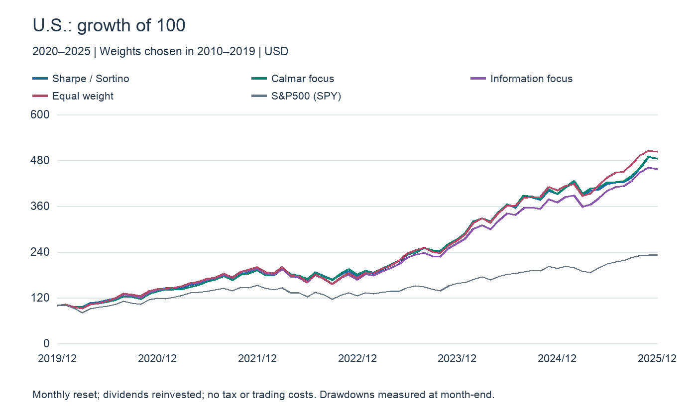
| Allocation | CAGR | Volatility | Sharpe | Sortino | Calmar* | IR | Max drawdown* |
|---|---|---|---|---|---|---|---|
| Sharpe focus | 30.06% | 17.50% | 1.604 | 3.129 | 1.945 | 1.188 | -15.46% |
| Sortino focus | 30.06% | 17.50% | 1.604 | 3.129 | 1.945 | 1.188 | -15.46% |
| Calmar focus | 30.09% | 17.06% | 1.642 | 3.272 | 2.012 | 1.232 | -14.95% |
| Information focus | 28.84% | 18.00% | 1.511 | 2.805 | 1.392 | 1.610 | -20.72% |
| Equal weight | 30.92% | 18.43% | 1.569 | 2.965 | 1.392 | 1.757 | -22.21% |
| S&P500 (SPY) | 14.99% | 17.13% | 0.905 | 1.465 | 0.627 | — | -23.93% |
*Volatility and ratios use monthly returns. Drawdowns and Calmar-style ratios use month-end valuations throughout. Wide tables can be scrolled horizontally.
In the later six years, the Calmar-focused allocation achieved Sharpe 1.642, Calmar-style 2.012 and a 14.95% maximum drawdown, with lower volatility than the Sharpe-focused candidate. Selecting a portfolio for a particular training objective does not ensure it leads that objective later.
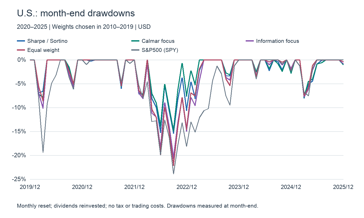
The information-focused portfolio’s subsequent information ratio of 1.610 beat the Sharpe-focused portfolio’s 1.188 but trailed equal weight’s 1.757. Equal weight nevertheless suffered a 22.21% month-end drawdown. Better benchmark-relative performance does not necessarily mean a gentler wealth path.
| Stock | Sharpe focus | Sortino focus | Calmar focus | Information focus |
|---|---|---|---|---|
| Toyota Motor (7203.T) | 5% | 13% | 13% | 9% |
| Mitsubishi Heavy Industries (7011.T) | 5% | 4% | 4% | 9% |
| Nintendo (7974.T) | 8% | 9% | 9% | 6% |
| Keyence (6861.T) | 25% | 25% | 25% | 23% |
| Shin-Etsu Chemical (4063.T) | 9% | 7% | 7% | 12% |
| Hitachi (6501.T) | 19% | 8% | 8% | 8% |
| Mitsubishi UFJ FG (8306.T) | 6% | 5% | 5% | 5% |
| Tokio Marine Holdings (8766.T) | 8% | 7% | 7% | 15% |
| Mitsubishi Corporation (8058.T) | 8% | 18% | 18% | 9% |
| INPEX (1605.T) | 7% | 4% | 4% | 4% |
Sortino and Calmar selected the same candidate in Japan, anchored by Keyence 25%, Mitsubishi Corporation 18% and Toyota 13%. The Sharpe candidate instead held Hitachi 19%; the information-focused candidate held Tokio Marine 15%.
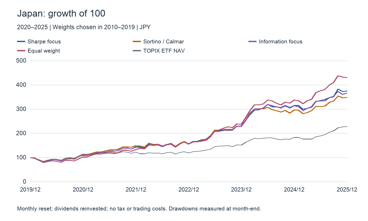
| Allocation | CAGR | Volatility | Sharpe | Sortino | Calmar* | IR | Max drawdown* |
|---|---|---|---|---|---|---|---|
| Sharpe focus | 24.60% | 16.68% | 1.412 | 2.836 | 1.235 | 1.136 | -19.92% |
| Sortino focus | 23.12% | 16.66% | 1.340 | 2.801 | 1.362 | 0.967 | -16.98% |
| Calmar focus | 23.12% | 16.66% | 1.340 | 2.801 | 1.362 | 0.967 | -16.98% |
| Information focus | 24.13% | 16.42% | 1.408 | 2.947 | 1.330 | 1.055 | -18.14% |
| Equal weight | 27.52% | 17.28% | 1.505 | 3.148 | 1.272 | 1.304 | -21.63% |
| TOPIX ETF NAV | 14.70% | 13.02% | 1.123 | 2.007 | 0.842 | — | -17.46% |
The Sortino/Calmar candidate’s maximum drawdown was 16.98%, versus 19.92% for the Sharpe candidate and 21.63% for equal weight. Its CAGR was 23.12%, below equal weight’s 27.52%. Equal weight also beat all four selected candidates on subsequent Sharpe, Sortino and information ratios. Optimizing a historical objective is not automatically better than a simple baseline.
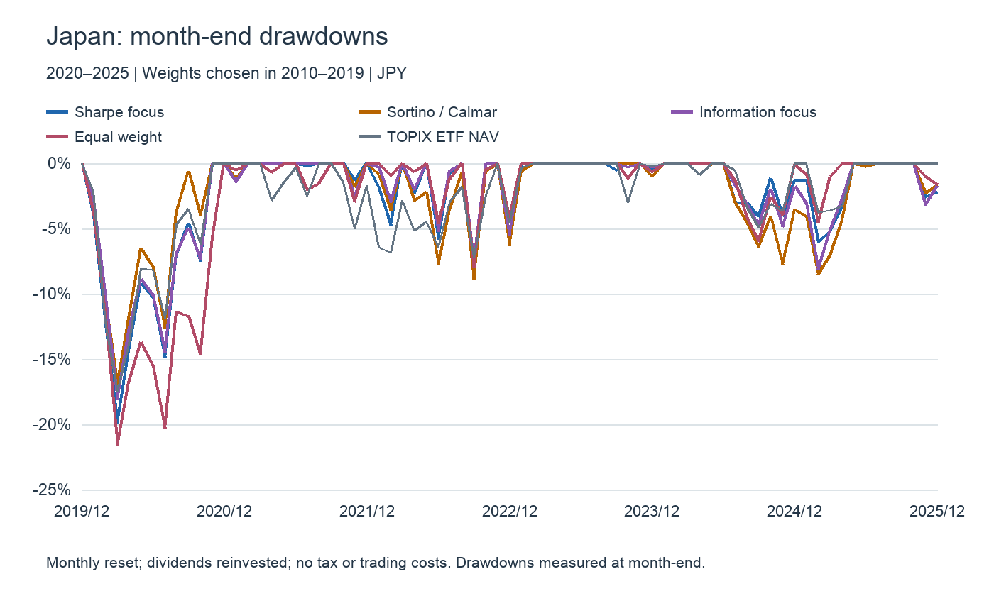
The TOPIX ETF reference had a 17.46% maximum month-end drawdown and 13.02% annualized volatility. Every selected stock allocation had a higher CAGR but also higher volatility. A high Sharpe ratio is not synonymous with low risk: the ratio and the level of risk answer different questions.
| Market | Objective | 2010–2019 | 2020–2025 |
|---|---|---|---|
| US | Sharpe focus | 1.708 | 1.604 |
| US | Sortino focus | 3.527 | 3.129 |
| US | Calmar focus | 2.020 | 2.012 |
| US | Information focus | 1.431 | 1.610 |
| JP | Sharpe focus | 0.799 | 1.412 |
| JP | Sortino focus | 1.289 | 2.801 |
| JP | Calmar focus | 0.494 | 1.362 |
| JP | Information focus | 0.832 | 1.055 |
This table compares each selected allocation on its own objective before and after the chronological split. The companies come from today’s site universe, not an investable historical universe containing delisted firms. The split prevents later returns from selecting weights, but does not remove the hindsight inherent in the stock universe.
Use Sharpe for overall variability efficiency, Sortino for shortfalls below an explicit target, Calmar-style measures and drawdown curves for peak-to-trough loss, and information ratio for benchmark-relative decisions. Choose the objective first rather than shopping for the most flattering statistic afterward.
These allocations provide comparison templates. Monthly trading in ten names incurs costs and potentially taxes; Japanese board lots can prevent exact integer-percentage replication. Compare equal weight with existing holdings before adding complexity. A quarterly schedule requires a new calculation rather than borrowing our monthly-reset results.
On the board, compare the S&P 500 or TOPIX with Lilly, Microsoft, Keyence and Hitachi. Intraday charts help distinguish company reactions from shared market news. Long-horizon measures evaluate the allocation as a whole; a single day cannot establish the long-run ratios used here.
For monthly portfolio return r and benchmark b: Sharpe=mean(r)/sampleSD(r)×√12; Sortino=mean(r)/sqrt(mean(min(r,0)²))×√12; information ratio=mean(r−b)/sampleSD(r−b)×√12. CAGR=terminal wealth^(12/n)−1; Calmar-style=CAGR/absolute maximum drawdown. Initial wealth 1 is included in the running peak. Month-end drawdowns omit intramonth troughs and are not daily drawdowns. Annualization uses the conventional √12 without autocorrelation correction. No trading costs, taxes or FX conversion. SPY uses adjusted market prices; Japan’s benchmark uses 1306’s distribution-reinvested NAV, not the TOPIX price index itself. Price history / 1306 manager
Data and references
- Nobel Prize: portfolio theory research history
- Sharpe (1994), The Sharpe Ratio; 1966 origins
- CFA Institute / Kidd (2012), The Sortino Ratio
- CFA Institute / Kidd (2011), The Sharpe Ratio and the Information Ratio
- Molyboga and L’Ahelec, Portfolio management with drawdown-based measures
- Yahoo Finance: dividend/split-adjusted stock histories
- Nomura Asset Management:1306 distribution-reinvested NAV history